Data Swamp

Data swamps are the result of mismanaged or unmanaged data lakes and an improper or non-existent import methodology. If you do not have a proper methodology when developing your data lake your data can become very messy or entangled, you can have duplicated data or orphaned data, expired or irrelevant data streams, improper data governance, controls, or permissions, or any other host of bad outcomes. Data swamps can take otherwise very well organized and managed information assets and turn them into inefficient and difficult to work with liabilities.

Data swamps can also alter the way you build the remainder of your information architecture in a negative way. Instead of being able to reduce your overhead by reusing existing processes or methods you will instead be in a constant battle with your improper architecture. You will be forced to adapt to the poor design which will only increase your technical debt and reduce your discretionary time. This could affect all your processes up and down your stack, become very costly to correct, and, at some point, it may even become impossible to fix.

The Data Universe - Measure Everything

The physical universe consists of physical matter and energy contained within a physical and time-bound space. The matter and energy within are governed and influenced by laws and competing natural forces which determine exactly how matter and energy can flow or exist within the universe. Because of these laws all possible movement and state of a given point of matter (such as an atom), are measureable and therefore predictable according to Newtonian Mechanics. Therefore, we can use the principles of Newtonian Calculus to track and measure the movement of matter within space and explain natural phenomena, such as the universal gravitational force.

Similarly, mathematical vector spaces can also act as a notional universe where points existing with a vector space are also bound by rules and mathamatical forces. This determines all the possible movements of those entites and also make it possible to measure the change of an entity's state within the vector space. This understanding can therefore be extended to include tracking the movement of matter over time within 3D Space.

Data Is Matter

So, how does this apply to data engineering? We believe that data is matter. Data exists as a physical entity bounded within a temporal universe and is therefore measurable according to the laws of Newtonian Mechanics. Data has a physical state, it exists somewhere, usually, at least in the cloud, this is in some sort of object storage, such as S3 or GCS, but the laws which govern the movement of data apply no matter where the data are stored. There are other caveats, such as data duplication, which we consider to be a logical untruth and a form of corruption. Truth, represented by data, can only exist in one point in a physical space and time universe, which is the entity's state.

To illustrate this point, lets consider a singluar datum, such as a user existing within an application. The user entity is of type class and has three fields:

user:class => ({
 uuid:string,
 name:string,
 type:string
})

It is interesting to note that although the class exists, it is still only a notional object. The object won't exist until it is actually instantiated by constructing the object. This code gives us a new user, Avril Stevens, by instantiating her as a type user. Note that "Avril Stevens" is not her primary identifier, that would be her UUID.

new_user:user => ({
 uuid:"ASip28sauioSAF",
 name:"Avril Stevens",
 type:"Customer"
})

As soon as this code is executed, the user datum "exists" within a physical and time bound space. We built the user at UTC timestamp "2023-06-07T06:07:15.324Z" and have her current state. This is also known as an event and is the basis of an event driven microservices architecture. Note that the timestamp is not a product of the user schema, it is a product of the creation event itself. In downstream processes these event timestamps will become part of the data model in support of data analytics and reporting. It is, of course, common to include this timestamp in the schema itself which is perfectly reasonable, but it isn't schematically or logically correct from a strictly transaction orientated consideration. The creation timestamp is a product of the creation event and is recorded as metadata, it is not a product of the user herself.

The datum instantitation from the user management service produces the create event and solidifies the current state of the user object at state_time:t0. This object can now exist as a key:value index within a datastore (such as bigtable or firestore) or an a row in a users table within an RDBMS. In essence, this datum now exists as matter within a 3-Dimensional space-time vector space (movement along a physical plane across a time vector).

Within an RDBMS system this is easily visualized. The datum must exist at one and only one physical address on disk, but of course, only within its current state. This is necessary to ensure referential integrity with other concurrent data logi stored within the data plane and is necessary to ensure ACID compliant transactions. This is why we recommend using an RDBMS such as cloud SQL or AWS RDS when performing transactions which must be absolutely guarenteed to be ACID compliant, such as financial transactions.

This understanding becomes more complicated within a cloud data store such as BigTable or Firestore. Here the datum is spread across multiple hard disks and across mutliple data racks and nodes. State management therefore becomes the responsibility of the driver of the service. The actual mechanics behing this is beyond the scope of this article, but the system has been proven mathamatically and logically true to represent a single unified "truth" of a given datum state, so we can assume this is correct for now. Even though the data exists across multiple physical addresses and disks, the systems management is effective enough at version management that it can ensure ACID compliance. Note that this is not an absolute ACID transaction where the object must be operated on in a single state. It is logically sound, but because the data is possible to exist in various states across various disks, it is not a true absolute ACID guarantee.

This becomes apparent when you examine the inner workings of a tool such as Cloud Spanner which attempts to manage concurrent writes across mutliple regional clusters to determine a singular truth-state of a given object. In the case of conflicting writes against a singular object spanner uses a voting mechinsm of multiple cluster states to determine democratically what the truest state of an object is. This is perfectly fine for almost all cases, but it is not the same as a singular entity existing on disk in an RDBMS. Indeed, when you examine RDBMS's such as AWS Aurora it consists of a singular writer node along with a number of reader nodes. The true state of the object is housed on the writer node only, and the reader nodes are eventually consistent against the writer node. The updates are usually perfomed extremely quickly, but it is still possible to read stale data from a reader node.

Within object storage, such as S3 or Google Cloud Storage, this becomes even more tenuous. Similarly to other cloud technologies object storage is replicated many times over across dozes or even hundreds of disks across regions, availabiltiy zones, racks, and nodes. This replication can take some time depending upon how the storage bucket is configured, such as storage tier, multi-region, and upon the size of the object being replicated. Object storage is 100% static on an object level. When an object is loaded into S3 it is always created as a new object. If you upload a same named object to S3 a new file is created and then S3 updates the pointer to the new file. This is why "updates" to objects take longer than creating a new file, and indeed can return stale data if the file is read before being updated. This is known as eventual consistency and has resulted in headaches for engineering teams working with data in S3. S3 is now "strongly consistent", which simply means that S3 requires verification of current object state before allowing an applciation to read the data. This works, but it isn't as fast as creating a new object, which is immediately available for reading. Additionally, although this solves for stale reads, it lacks certain qualities that are useful to data engineering, such as version tracking or state management.

ACID Transactions in the Cloud

It is worth pointing out that, technically, there is no true concept of a primary key in cloud data warehouses because a primary and foreign key relationship in the context of RDBMS technically refers to data storage addresses in a standard block storage (hard drive). Cloud data warehouses use distributed object storage, so the concept of a primary key or foreign key doesn't exist and is not enforced within a cloud data warehouse. Some cloud data warehouses allow you to "declare" a primary key or foreign key on a table, which can help with query planning, but we consider this a misnomer since it doesn't have the proper referential integrity constraints nor distinct key requirements to be a true primary key. It would be closer to a query hint than to a primary key. In the proceeding text we will note instances of "primary keys". This should be taken to mean the qualities of the data which positively identify a unique row within a table, such as event-timestamp, and is not a true physical primary key.

It is still possible to utilize the concepts of primary and foreign key relationships to build our data models. the logical application of keys is still valid, they're just not enforced within cloud data warehouses. This also means that multi statement transaction integrity is not really possible within cloud data warehouses either, at least not in its familiar form. Google is working on a method for transaction handling within BigQuery. Redshift has a method which produces "an illusion of a transaction", which effectively produces locking and transaction simulation, but this isn't a true transaction like what you would get from an RDBMS. If transaction or relationship integrity is absolutely required for your workload then cloud data warehouses might not be the best answer and a standard RDBMS might be a better option. Providers are getting close to ensuring ACID transactions, likely through clever storage manipulations and version management, but it is not the same logical transaction mechanism as found in RDBMS. For more information on why ACID transactions are so difficult in the cloud see this wiki on the CAP theorem. The data universe approach helps facilitate row-based transaction handling in the cloud by focusing on time as our universal solvent.

We solve this issue by processing entire tables or partitions all at once and by completely rebuilding data sets with each run. By taking advantage of time-space partitioning we can most readily and most generally "zero-in" on key points of data or new data in order to minimize processing costs and ensure dataset integrity throughout the warehousing process.

The Data Universe Architecture

We've established that data are matter, and we've agreed upon a common set of principles to ensure object consistency in the cloud. So how can we now ensure data consistency and version tracking for objects stored within a data lake? We like to use the data universe strategy to our advantage. This means that we embrace the notion of data existing within a 3-Dimensional vector space where a data has a location in space, such as an object storage URI, and that object has the potential to mutate over time, and that these mutations are useful and relvant information for the data engineer to capture and maintain. These mutated states exist along a timeline and against a physical prefix and address in cloud storage.

These objects are not necesarily the absolute source of the true object state, which likely exists within a transactional database, but these are object instantitations captured at a given state at time t=n. Our objective is to capture these mutations and allow our system to parse through them in order to positively identify their state and effectively report on the information contained.

The general structure is heirarchical and goes from the "highest" level of your data to the "lowest". This is effectively forming your data catalog and will make it very easy for cloud data warehouses to find and parse through your data. This structure allows any warehouse to find the data that it needs by searching the file name (URI) only and the warehouse will not have to open/read the file to sort through the data. This will become very useful when we begin to model our data. This methodology is effective for either batch or micro-batch data.

With this structure we can now confidently say a few things:

• The data we expected to receive this morning has arrived (local date).
• We know exactly which data came today (the timestamp is your de facto import id).
• We can easily compare the data from today with imports from other days.
• We only have to pull this instance's data to complete our delta processing (hive partitioning).
• We have an exact timestamp we can use for auditing or when communicating with third parties.

This method allows for multiple imports per day because of the timestamp partition. You could run it as often as you would like throughout the day, and you could actually get very close to streaming near real-time data using this method as well, though this method is best suited for batch or microbatch data. This method is very flexible and allows for a wide range of choices for how to execute against a wide variety of data sources effectively and efficiently.

When using a federated table or external inside of a data warehouse, the data are available for querying as soon as they land in cloud storage. We still prefer to add another step to materialize the data into a table for performance reasons. This requires transformations to clean and correctly type the data.

Once we start building our data warehouse, we will bring this metadata forward and it will become very useful for a variety of use cases (such as historical analyses or building slowly changing dimension tables).

External Table Conceptualization

The overall architectural objective is to effectively translate external data structures into useful and consistent schemas in order to begin modelling and profiting from our data assets. For now, the focus is on conceptualizing a faithful representation of our external data inside of our data warehouse so that data modelling and table instantiation can begin.

The import schema houses an ephemeral copy of your raw data stored within the data lake. It is essentially a reflection of your data lake, technically it is your bridge between your data warehouse and data stored within the data lake.

Data Universe Translation

This brings us back to the notion of a data universe as the general structure of our data lake. Data modelling in the cloud takes advantage of a data system which is partitioned along a mass-time vector space. The general folder structure of the data universe for batch data is:

and for streaming:

The folder structure itself will form the basis of our entire data warehouse. The Unix epoch is the import timestamp, which is also the import id. Using this method our primary identifier of the table within our data universe essentially takes on mass and time, allowing vectorization and associated vector space transforms:

When data is considered to be a physical property which exists within space-time it becomes possible to perform advanced analytical calculus on the table in order to measure change against data points and values. This can be useful for measuring time series derivations within data, such as 1st and 2nd order derivatives for financial assets.

This another great example of the power of the cloud. Previously, capturing and maintaining continuous instance definitions of data assets would be massively expensive and time consuming. With the huge economies of scale and standardized tooling available with cloud computing technologies it is now feasible for almost any company to effectively and properly manage their historical data.

Data Surfacing and Partitioning

Given our data universe folder structure we begin the process of surfacing our data in the data warehouse. This is done by building hive partitioned external tables in BigQuery or in Redshift by creating partitioned external tables. The process is slightly different for either system, but the effects are the same. The next step is to surface the data as string types only. We will then build a view which will give us the correct data types, and finally we will load this as a true table in the data warehouse translation layer. The data should be partitioned by dt={date} and ts={int64} for batch data or dt={date} only for streaming data. The partitioning will allow us to effectively parse the data to zero in on a particular import timestamp or easily access the most recent data.

When developing the external table for delimited data you should set all columns to string data types first, even if you know for sure what the data types are (always assume there will be errors in the data until proven otherwise!). If you try to set data types for the columns and there is an error in the data then you will have to scrap the table and start over.

For JSON data we will treat the whole Json object as a single column. This means that you actually surface JSON data as a delimited file with only one string column. If this is event data from a system such as Pub Sub your external table would be a character delimited file with a character delimiter and three string columns.

Cleaning, Typing, and Instantiating the Data

Now that the import table is present in the import layer of our data warehouse we can move to the cleaning and translating phase. The goal of this phase is to properly clean, type, and instantiate the data into a materialized collection table.

It is essential to properly clean, type, and instantiate the data so that it becomes much easier for the warehouse to perform calculations and create query plans within the data warehouse. It is also helpful when developing data catalogs or other metadata repositories.

Temporal Targeting and Delineation

With the data universe strategy, the data are partitioned along the local HQ date and contain the UTC timestamp either as an additional prefix for batch transactions or as part of the filename for streaming data. With this method it becomes feasible to target individual points in time within the matrix.

To take advantage of this we will build a view on top of the external import table you just built. At this point you will still want to treat the columns as strings, but it can be prudent to extract the event timestamp from here as well (remember that the timestamp we have in our prefix is import timestamp, not event timestamp). Additionally, you'll want to extract the data lake prefixes as import_date_local and then convert the timestamp (either the prefix for batch or the filename for streaming) as import_timestamp_utc. It is essential to extract theses values to effectively parse through the data and retrieve the most current data as well as account for any duplicates. The import timestamp (aka the "current as of" timestamp) is a unique identifier, whereas the event timestamp can be the same day to day for data points which aren't updated often. Generally, you'll want both.

Most use cases want to look at the most current iteration of the data. Include this in your WHERE clause WHERE dt={current_date} to access the current day's data. This will limit the query to the current day's data which will help keep costs down. It is also possible to target specific timestamps using WHERE ts [=, <, >] {timestamp_utc} if you want to pick up your data from the last imported record or you want to target an individual batch or record.

If you only import the data once per day then this is sufficient, however if you import the same data points multiple times per day then there is one more step. In the query add a select for a row partition along the event-id and then sort the rows descending by the import_timestamp. It should look like SELECT ROW_NUMBER() OVER(PARTITION BY <event_id> ORDER BY ts DESC) as row_ Then create a wrapper query on top of your original view which includes the filter WHERE row_ = 1

Cleaning and Typing Delimited Data

It is much easier to work with transformations inside of SQL and within the data warehouse than within another process such as python. This is why the first step was to create an import table with only string columns. For delimited data the process is fairly straightforward, but it can become overwhelming if the data are full of errors.

The goal is to create a reflection of your data lake in the cloud data warehouse. Begin by identifying the correct data types and column names. The best way to clean your data for an import table is to identify the data points that do not fit your model. So for each column run a SQL statement with WHERE <column> IS NOT NULL AND SAFE_CAST(<column> AS <data_type>) IS NULL Use this same method to identify any dirty data in the table. Use WHERE <column> IS NULL to identify any missing data.

Once any dirty data have been identified you must write SQL code to clean the dirty data and get them into the correct type. This can be a very tricky process if there are a lot of errors in the data, but for the most part errors usually occur in some sort of pattern which is conducive to SQL. You can use chained transformations to break up the cleansing logic into manageable pieces.

Cleaning and Typing JSON Data

JSON data (usually unstructured event data) is more complicated to clean and type, but the essential processes are the same. The trick is to break the string data into manageable pieces and then recombine them after cleaning. Some systems offer schema inference, but this only works if the schema never changes. If the schema are divergent or the data is dirty in some way we can accomplish shematization through SQL native JSON parsing and chained transformations.

Given the above links to detailed explanations of the transformation tools we will jump into cleaning and typing the substrata of the descendent JSON object.

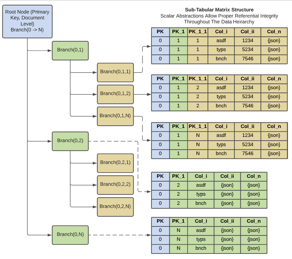
For each given JSON superstrate, break the substrate along table key delimiters to reveal the submatrix definition while maintaining referential integrity with the host superstrate. Be sure to break the JSON into its lowest-level, foundational substrata. Within a view of each individual substrate the data points form columns along the constant determinates of the ascendant superstrate. For each column within the isolated substrate view use SQL statements to properly clean and type the data similarly to the above logic used for the delimited data.

All substrate views are delimited against ascendant table keys. Use built-in JSON aggregation techniques to reassemble the cleaned view along table key aggregators (For Redshift, use LISTAGG). Roll up all substrate into the superstrate of the descendent objects. Continue this until you have reached the root level object containing all descendent logic summed up in the Σx select of your chained transformation. Essentially, this is the inverse process of the JSON parsing methodology.

The end result of this process will be a fully formed, typed, and cleaned view with proper nested and repeated fields representing the whole of your JSON object.

Table Instantiation

At this point this is still technically import data, and we want the materialized table to reflect the data lake and current day operations. You will still want to partition the data by the local import date. If you import the whole dataset all at once every day then this process is simply to replace the materialized data from the day before by executing a SELECT * against the view you created above.

It is possible to rebuild the entire dataset by removing the dt={current_date} filter from the temporal targeting view. Though this is usually only used when a complete rebuild is necessary or this is the initial table construction. If your data are small enough this is certainly an option you could run daily.

If the data are ran multiple times per day you can target the most recent updates by converting the import_timestamp_utc column in the materialized table and including WHERE ts > (SELECT MAX(UNIX_SECONDS(import_timestamp)) FROM <import_table>) in the temporal targeting table view. it is also possible to use WHERE import_timestamp_utc > (SELECT MAX(import_timestamp_utc) FROM <materialized_table>) in the final view. If you want to save the most money by targeting individual timestamps you would have to first have to save the results of the query (SELECT MAX(import_timestamp_utc) FROM <materialized_table>) as a variable and then pass that variable to the WHERE clause in the targeting view. This of course means that you will now be executing a stored proc instead of simply a view. This is just a quirk of Dremel and is likely due to the lack of true transaction handling in the cloud.

When building your materialized tables it is now possible to partition this data on the import_timestamp, local import date, or event_timestamp_utc. You can also set partition expirations for housing shorter term data to save on costs. Sort your data by the event_timestamp_utc or import_timestamp to get improve query performance when building clustered tables.