Delimited File Parsing and Transformations

This article discusses our method for creating exteral tables for character delimted data. Importing, cleaning, and properly typing incoming delimited data is a fundamental task of data engineering. This article assumes that a data lake and import process have been created already and data are flowing into storage.

Creating an External Table

The first step is to develop an external table inside of BigQuery which contains the reference instructions to query the data inside of GCS. Google details the proper method for building the externally partitioned data in their documentation.

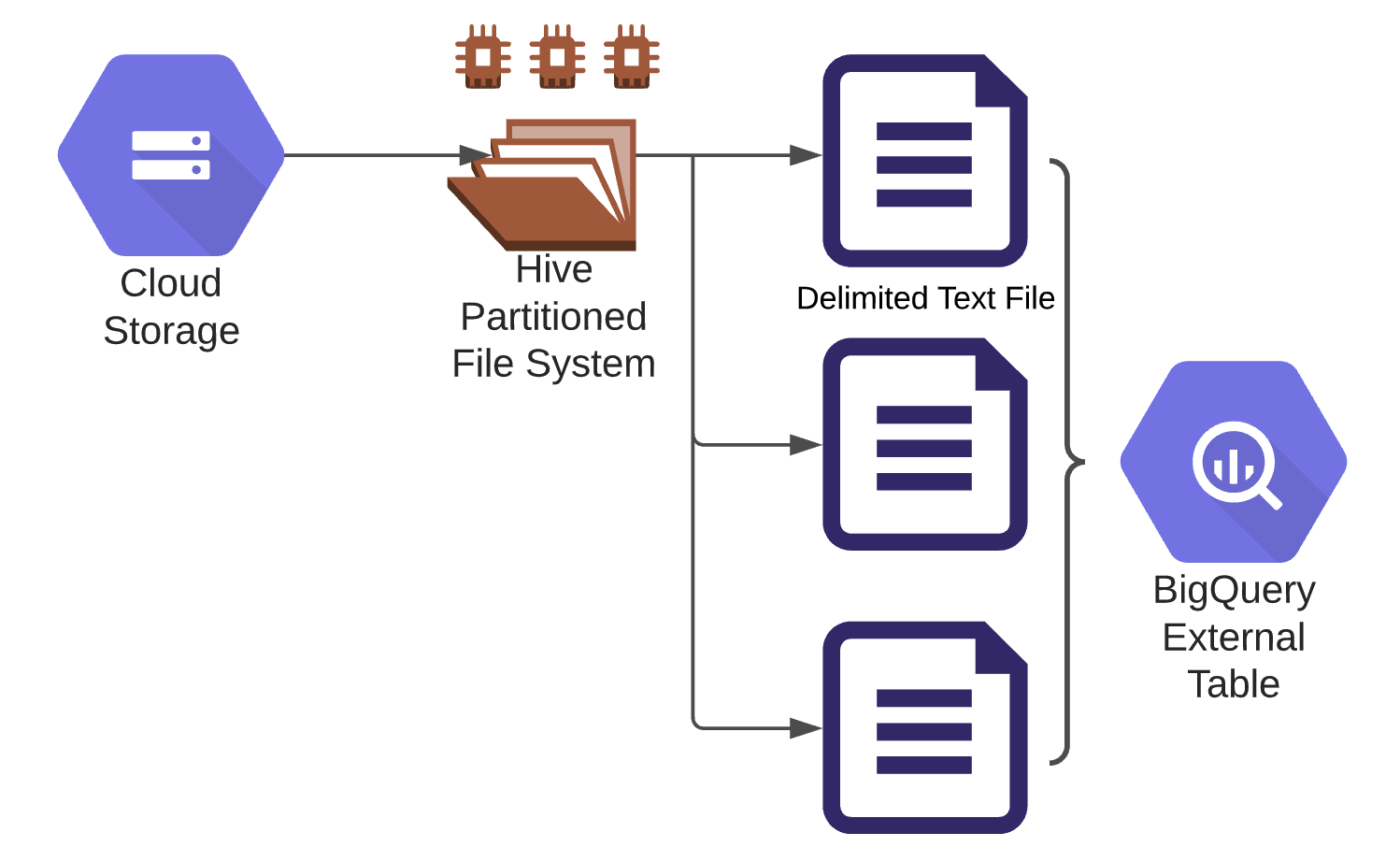
We often see errors or incompatible data types in data files, especially from unknown or outside sources. Attempting to build a table schema with proper typing directly oft en leads to import errors. We recommend building import schemas using all strings and then building a transform view on top of the import schema.

Transformation and Load via Chained Transformations

After successfully setting up the external table the next step is to create the transformation logic. We build the transformation logic using a series of ctes (or views) and then the final result set is materialized as a table.

We call this "chained transformations". This method is useful because it gives us a single script to reference all transformations and to build the end table. At this point our only objective is to solidfy a cleaned and typed abstraction of the host datalake object within the data warehouse.

SQL Native JSON File Parsing

Parsing and transforming imported raw new line delimited JSON data is often a tricky task because the schemas are often ambiguous and can change often. This is especially true when working with dynamic data across multiple applications. Therefore, we have devised a general solution to parsing any possible JSON data using any given data warehouse, as long as the data are functionally complete object abstractions (meaning they faithfully represent real world events). Of course, due to the heavy processing requirements needed this method works best on a cloud data warehouse such as BigQuery or Redshift.

While BigQuery does have a schema abstraction tool and automatic schema identifier we find that this is almost always insufficient as just one import error in your model will result in a total failure of the read with very little error details. We have found a more robust method for parsing and modeling the data within BigQuery.

Creating an External Table

The first step is to develop an external table inside of BigQuery which contains the reference instructions to query the data inside of GCS. Google details the proper method for building the externally partitioned data in their documentation.

Creating the table schema is similar to character delimited data, however, for delimited JSON data we will create a table schema with only one column for a json item. Occaisionally there are multiple columns associated with the data as well as the JSON data itself. These columns can include a primary key, such as a message id and a timestamp, or any other combination of columns. This is perfectly compatible with our method. JSON data "descends" from a primary identifier.

This method requires treating the json data as a character delimited file (not as a json delimited file). This means that you treat the JSON data as just another column in the file.

JSON Parsing Formulae

This is where things start to diverge from character delimited files. Json is not demarcated by character qualifiers, but is an abstracted multilayer and multidimensional schema nested within a single string. SQL wants to work with tablular (two dimensional) data, but JSON is multidimensional, ambiguous, and subject to change. In order to properly qualify this data we need to parse each layer of the JSON into individual tables while maintaining referential integrity to the source data. The effort is to build a matrix of the data which contains abstract scalars that are effective array-key identifiers of the tabular data.

This differs from the "standard approach" of json parsing where you are required to map out lengthy and convoluted JSON address id's in order to pull data into a table. Some of the advantages to this approach include:

Access to multidimensional data sets within a column-oriented querying approach

Parsing individual pieces of the data seperately to minimize errors and ease debugging

Easy normative references to higher and lower chained abstractions within the JSON data heirarchy

Easy adaptation to changing schemas or data types

Robust extraction architecture which minimizes or eliminates common import errors

Easy reference architecture and transformations

Similarly to charcter delimited text files this will consist of a series of views which will eventually be materialized into a table. However, whereas delimited text files are essentially two dimensional objects which require a simple straight line path from source to target, JSON files often require complex abstractions along multiple branching paths. We must "break apart" the file into its individual components and then "reassemble" the pieces into our prefered model. It's somwhat similar to dissasembling a jigsaw puzzle, refashioning all the pieces, and then rebuilding it.

Disassembly and Mapping

JSON data is heirarchical and multilayered and consists of several data types. These include strings, numbers (ints and floats), arrays, and subcollections. Any solution devised will have to be able to faithfully replicate the data schema inside a BigQuery table. Below is a general breakdown of an example JSON object (document). The data are separated into two dimensional arrays (tables) demarcated by a unique scalar which identifies array positioning and document mapping instructions for reassembly.

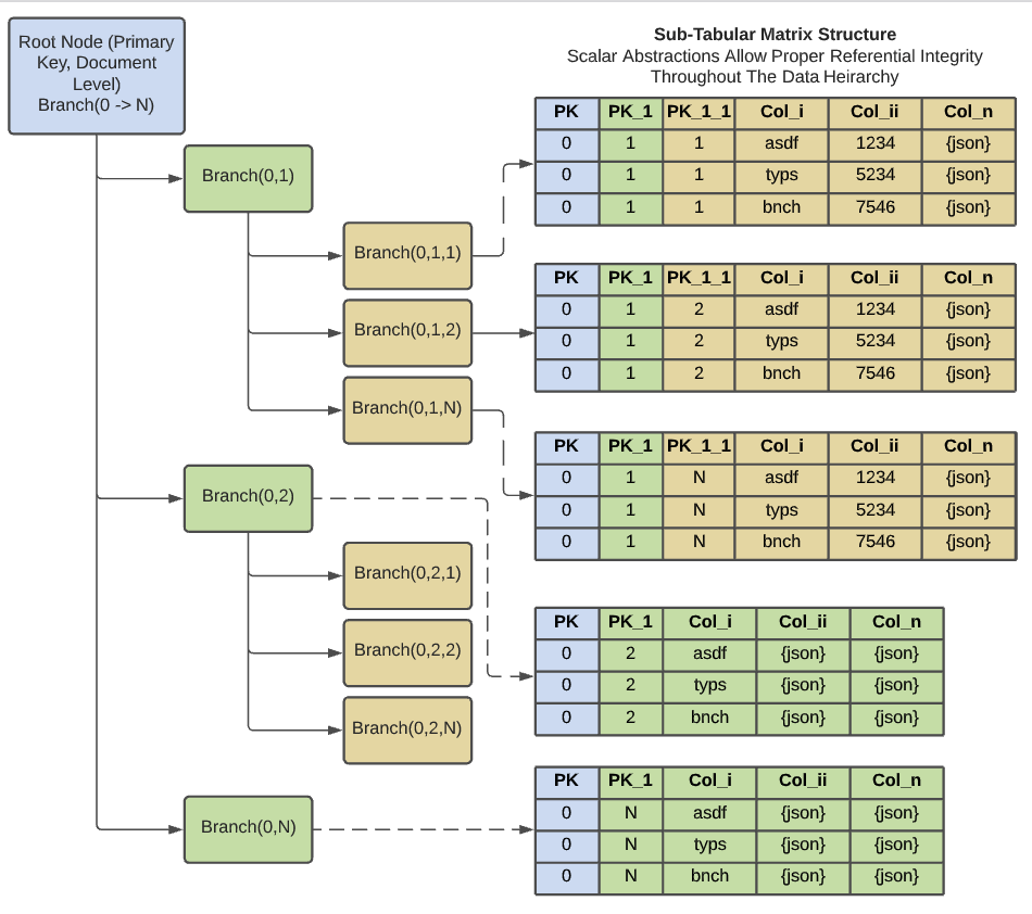
The identifier is essentially a scalar which can be thought of as a sort of pointer within the vector space. To dissasble the data we break the data down along the unique identifier. These identifiers consist of a primary key along with scalar indicators demarcating JSON heirarchical depth. At the root level we have a primary key which uniquely identifies the JSON string being broken down. Usually, this is a message identifier indicating an application message or an elasticsearch object id. If there is no primary key then a row number can be used instead, as long as there is a way to uniquely identify the row.

Array indicators are assigned to individual sub collections as they are broken down. The array indicators are row numbers partitioned against the higher level primary key identifier and along the descendant objects. Array key identifiers are aligned to column names demarcating the subcollection depth.

For example, this could be:

and so on until the maximum depth is reached. We find it a best practice to use the names of the immediate parent key being parsed as the descendent column names.

Use a simple JSON key extraction function to pull the key names out from a sample of the data with each level pulled. Stack Overflow has some good examples for how to do this in BigQuery. Use the keys to build each individual table schema and type them as strings for now and without any transformations.

Each table or subcollection gets its own view as shown in the subtable mapping. These views should contain the primary key identifier, all descending array keys, and any columns mapped as string datatypes (including any JSON attached to the table). This system is highly adaptable to changing schemas or datatypes as it is very easy to update the model with any new columns. If a JSON string does not contain a given column then the system simply assigns a NULL value to the column.

Reassembly and Materialization

After the data is appropriately mapped and parsed into the appropriate views we can now move to the build phase. The build phase is a reassembly methodology designed to properly materialize tabulted JSON data into correlating BigQuery tables. Data from the disassembly and mapping above is technically querable in it's current format, but to get the most efficient queries from BigQuery with this data we should rebuild and materialize the table appropriately.

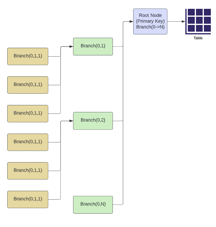
The integration process involves rebuiling the tables by essentially recombining the data which was previously parsed out by using SQL joins and stuct rebuild processes. Tables are joined along the primary key and array key identifiers. As we broke the original data down from top to bottom we must rebuild it from bottom to top by rolling the data up to the higher level dimension. Eventually, the entire data model can be rebuilt and materialized properly in BigQuery which will allow proper and efficient queries.

To recreate the objects faithfully use the struct object in BigQuery and build the model as a CTE. Ensure that the data are properly typed and formatted when executing the rebuild objects. The data are rolled up to the higher level object and this object now assumes the proper data typing and structure of subcollection objects.

Continue to roll up all the objects in this method until the top level dimension is reached. At this point we now have the proper data model created and can push this data into a BigQuery table. When set up correctly this is a highly stable and efficent method of parsing and mapping JSON data within BigQuery.